改造は人の業

ラッパー関数を作る

f <- function(a) a + 1 

f_hex <- 
  function(hex = "f") { # 引数名変更 & 初期値設定
    strtoi(hex, 16) %>% # 前処理
      f() %>%
        as.hexmode() # 後処理
  }

f_hex("a") # [1] "b"

名前空間に殴り込む

assignInNamespace()

• メリット
  • 内部変数を弄ることも含め、何でもできる
  • formals が対象なら便利なパッケージがある
    (hoxo-m/fixer)
• デメリット
  • オブジェクト間の依存関係による予期せぬ副作用

関数の構成要素を魔改造する

formals() を弄って

assignInNamespace() せずに

内部変数も含めて挙動を弄ろう

インストール & 読み込み

devtools::install_github(
  "atusy/presentation",
  subdir = "japanr2018/pkg"
)

library(japanr2018)

中身

#' An internal variable
#' @noRd
b <- 1

#' An exported function
#' @param a A numeric vector
#' @export
f <- function(a) a + b

#' An function depending on f
#' @inheritParams f
#' @export
g <- function(a) f(a)

namespace:japanr2018 に隔離

f
# function(a) a + b
# <bytecode: 0x3e05f08>
# <environment: namespace:japanr2018>

f <- 1
f
# [1] 1

japanr2018::f
# function(a) a + b
# <bytecode: 0x3e3d700>
# <environment: namespace:japanr2018>

japanr2018::f は上書きされない

formals() で関数の引数を確認する

str(formals(japanr2018::f))
# Dotted pair list of 1
# $ a: symbol 

ヘンなリストだけどリストのノリで弄れる。

弄るには`formals<-`

f <- japanr2018::f
formals(f) <- list(a = 1)
formals(f)

## $a
## [1] 1

f()

## [1] 2

alist() を使うと遅延評価できる

f <- japanr2018::f
(formals(f)$a <- alist(a = rnorm(1))$a)

## rnorm(1)

f()

## [1] 3.439521

f()

## [1] 0.649811

?formals にも載ってるアブナい技

確認

japanr2018::f

## function(a) a + b
## <bytecode: 0x4b4b6f8>
## <environment: namespace:japanr2018>

japanr2018:::b

## [1] 1

b を a と同じ長さの乱数にしたい

f <- japanr2018::f
formals(f)$b <- alist(b = runif(length(a)))$b
f(1:3)

## [1] 1.438568 2.591437 3.015478

f(1:4)

## [1] 1.994207 2.425113 3.596890 4.074767

たし算じゃなくてかけ算がいい

f <- japanr2018::f
formals(f)$`+` <- `*`
f(1)

## [1] 1

japanr2018::g は影響を受けない

japanr2018::g(1) # g = function(a) f(a)

## [1] 2

assignInNamespace("b", 2, "japanr2018")

していたら

japanr2018::g(1) == 3

になっていた

ggproto で StatCI を定義

StatCI <- ggproto(
  "StatCI",
  ggplot2::StatDensity,
  compute_group = function(data, self, ci = 0.95, bw, adjust, kernel, n, trim, ...) {
    # calculate density based on StatDensity
    res <- self$super()$compute_group(
        data = data,
        bw = bw,
        adjust = adjust,
        kernel =kernel,
        n = n,
        trim = trim,
        ...
      )

    # quantile intervals to trim res
    Q <- quantile(data$x, 0.5 + ci / c(-2, 2))
    L <- Q[1] <= res$x
    U <- res$x <= Q[2]

    # return trimmed res
    rbind(
      find_boundary(res, !L, Q[1]),
      res[L & U, ],
      find_boundary(res, U, Q[2])
    )
  }
)
find_boundary <- function(data, bool, lim) {
  if(any(data$x == lim)) return(NULL)
  neighbors <- data[sum(bool) + c(0, 1), ]
  colSums(neighbors * rev(abs((lim - neighbors$x) / diff(neighbors$x))))
}

ggplot2::stat_density() を
stat_ci() に改造

ggplot2::stat_density # コピペ & 目sedは嫌だ

## function (mapping = NULL, data = NULL, geom = "area", position = "stack", 
##     ..., bw = "nrd0", adjust = 1, kernel = "gaussian", n = 512, 
##     trim = FALSE, na.rm = FALSE, show.legend = NA, inherit.aes = TRUE) 
## {
##     layer(data = data, mapping = mapping, stat = StatDensity, 
##         geom = geom, position = position, show.legend = show.legend, 
##         inherit.aes = inherit.aes, params = list(bw = bw, adjust = adjust, 
##             kernel = kernel, n = n, trim = trim, na.rm = na.rm, 
##             ...))
## }
## <bytecode: 0x5fe15d0>
## <environment: namespace:ggplot2>

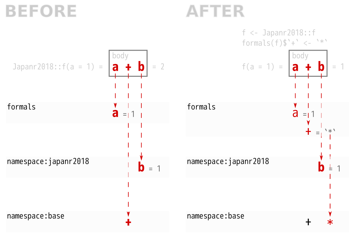
stat_density() が呼び出す StatDensity を、
ggplot2::StatDensity から、引数の StatDensity に摩り替え

library(ggplot2)
stat_ci <- stat_density
formals(stat_ci) <- c(
  formals(stat_ci), 
  StatDensity = ggAtusy::StatCI
)
ggplot(data.frame(x = rnorm(1e5)), aes(x)) +
  geom_density() + stat_ci()

実際には StatDensity 引数を弄れないよう、もう一工夫した。

Disclaimer

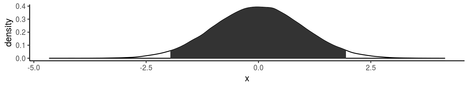
遊び半分の実装です。

実用的には ggdistribute や bayseplot があります。

内部変数 skimr:::optioins を弄る

library(skimr)
skimr::inline_hist(iris$Petal.Length)

## ▇▁▁▂▅▅▃▁

myopt <- rlang::env_clone(skimr:::options)
inline_hist <- skimr::inline_hist
myopt$formats$character$width <- 20
formals(inline_hist)$options = myopt
inline_hist(iris$Petal.Length)

## ▁▇▂▁▁▁▁▁▁▁▃▃▃▅▂▃▂▁▁▁

動的に optioins を弄る

inline_hist <- skimr::inline_hist
.options <- function(n) {
  options <- rlang::env_clone(skimr:::options)
  options$formats$character$width <- n
  options
}
formals(inline_hist)[c("n", "options")] <- 
  alist(n = 10, options = .options(n))

inline_hist(iris$Petal.Length)     
# ▇▃▁▁▂▆▆▃▂▁
inline_hist(iris$Petal.Length, 20) 
# ▁▇▂▁▁▁▁▁▁▁▃▃▃▅▂▃▂▁▁▁

S3メソッドを手抜きして作る

print.atusy <- function() {
  cat("Printing atusy class object.\n")
  NextMethod()
}
formals(print.atusy) <- formals(print)
structure(1, class = "atusy")

## Printing atusy class object.
## [1] 1
## attr(,"class")
## [1] "atusy"

S3メソッドは最低でも、
総称関数と同じ引数を持たなければならない

`formals<-`() を使えば総称関数の引数を丸々引き継げる